Deep Reinforcement Learning for Blackjack

Earlier experiments showed how an RL agent can learn basic strategy, adapt to real casino rules, and rediscover card counting by scaling bets with deck composition. This final step uses a neural network to approximate Q-values, enabling generalization across a much larger state/action space and combining both betting and play decisions.

Environment and State

The environment provides a fixed-length numeric observation vector that encodes both phases and the count:

def _obs_vector(self):
    """
    Return a fixed-size numeric vector for DQN:
     [phase_play,               # 1 if play-phase, 0 if bet-phase
      player_total_norm,        # /21 (0 if bet phase)
      dealer_up_norm,           # /10 (0 if bet phase)
      usable_ace,               # 0/1
      allow_double,             # 0/1
      true_count_bucket_norm,   # bucket / max(|min|,|max|)
      bet_norm]                 # current bet / max(BET_OPTIONS)
    """

def _obs_vector(self):
    """
    Return a fixed-size numeric vector for DQN:
     [phase_play,               # 1 if play-phase, 0 if bet-phase
      player_total_norm,        # /21 (0 if bet phase)
      dealer_up_norm,           # /10 (0 if bet phase)
      usable_ace,               # 0/1
      allow_double,             # 0/1
      true_count_bucket_norm,   # bucket / max(|min|,|max|)
      bet_norm]                 # current bet / max(BET_OPTIONS)
    """

This lets the network reason jointly about play context, dealer strength, doubling eligibility, and the true count signal driving bet sizing.

Deep Q-Network (DQN) with Valid-Action Mask

The network outputs Q-values for all actions (bet actions during the bet phase; hit/stand/double during play). Not all actions are legal in every state, so the TD target masks invalid actions:

def compute_td_target(q_next, mask_next, rewards, dones):
    """
    q_next: [B, A], mask_next: [B, A]
    target = r + gamma * max_a' q_next(s', a' allowed) * (1-done)
    """
    # set invalid actions to -inf so max ignores them
    q_next_masked = q_next.clone()
    q_next_masked[mask_next == 0] = -1e9
    max_next, _ = q_next_masked.max(dim=1)
    return rewards + (1.0 - dones) * GAMMA * max_next

def compute_td_target(q_next, mask_next, rewards, dones):
    """
    q_next: [B, A], mask_next: [B, A]
    target = r + gamma * max_a' q_next(s', a' allowed) * (1-done)
    """
    # set invalid actions to -inf so max ignores them
    q_next_masked = q_next.clone()
    q_next_masked[mask_next == 0] = -1e9
    max_next, _ = q_next_masked.max(dim=1)
    return rewards + (1.0 - dones) * GAMMA * max_next

This preserves blackjack rules (e.g., Double only when allowed) while stabilizing learning with a target network, replay buffer, and ε-greedy exploration.

Training Progress

Below is the exact training log snapshot from a 150k-episode run:

Ep   5000 | EV -0.0068 | W/P/L 0.438/0.092/0.470 | ε=0.193
Ep  10000 | EV -0.0427 | W/P/L 0.429/0.081/0.490 | ε=0.187
...
Ep 145000 | EV -0.0035 | W/P/L 0.434/0.091/0.475 | ε=0.020
Ep 150000 | EV -0.0333 | W/P/L 0.422/0.086/0.491 | ε=0.020

Ep   5000 | EV -0.0068 | W/P/L 0.438/0.092/0.470 | ε=0.193
Ep  10000 | EV -0.0427 | W/P/L 0.429/0.081/0.490 | ε=0.187
...
Ep 145000 | EV -0.0035 | W/P/L 0.434/0.091/0.475 | ε=0.020
Ep 150000 | EV -0.0333 | W/P/L 0.422/0.086/0.491 | ε=0.020

Observations:

• EV fluctuates but tends toward small negatives as ε decays.
• Win/push/loss ratios remain realistic (~42–44% wins, ~8–9% pushes, ~48–50% losses).
• Late checkpoints hover close to break-even, notable given the expanded action space.

Training Loss and EV Curves

To better understand stability, two curves are tracked during training:

1. Training Loss (Moving Average):
   Shows how well the network’s Q-value predictions align with observed returns.
   Expected behavior: noisy early training, then stabilization as policies converge.
2. EV over Training (Greedy Policy):
   At evaluation checkpoints, the greedy policy’s expected return is estimated.
   This highlights how exploration decay (ε → 0.02) affects final strategy quality.

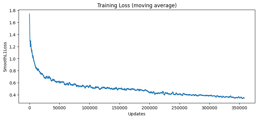
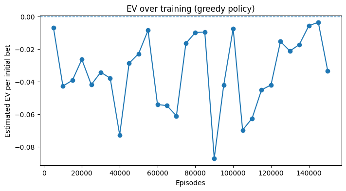
Typical runs show high loss variance in the first 20k episodes, then a downward trend. EV estimates follow a noisy trajectory but settle in the −0.01 to −0.05 range, consistent with professional-level play but still negative given house rules.

Final Policy Snapshots

First-decision tables display human-like structure:

• Hard totals: stand on 17+, stand more often against weak dealer upcards, hit vs strong ones.
• Soft totals: aggressive doubles in favorable conditions, especially as the count improves.
• Betting: larger bets in positive true-count buckets.

Conclusion

• A vectorized state and masked DQN update allow the agent to jointly learn play and betting while respecting blackjack rules.
• The learned strategy mirrors professional intuition: stand on strong totals, double selectively, and raise bets when the count is favorable.
• While EV remains slightly negative, the agent demonstrates the core behaviors of real-world advantage play—learned entirely from interaction, without hardcoded rules.