Neural Networks Part 1: Teaching a Neural Network to Learn Math

Can a Neural Network Learn to Think Like a Calculator?

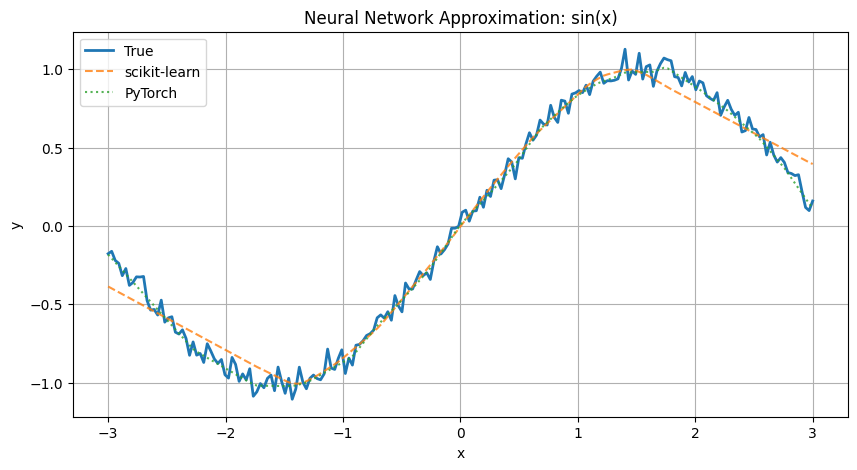
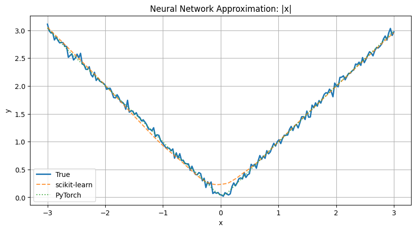
Neural networks have become one of the most powerful and flexible tools in modern machine learning. But how do they actually learn — and can they really approximate things like a calculator? In this first post of our three-part series, we introduce neural networks in a hands-on way by showing how they can approximate simple mathematical functions like:

• y = x², 
• y = sin x
• y = |x|

We’ll use both scikit-learn and PyTorch to compare implementations.

A link to this notebook and the other notebooks can be found here on GitHub

Why This Matters

Before using neural networks for pricing complex financial instruments, it’s important to understand what they actually do. These experiments demonstrate a foundational concept:

Neural networks can approximate unknown functions simply by observing input/output examples.

Even when you don’t tell the model the underlying equation, it can figure out the shape of the function by training on data — this is why they’re often called universal function approximators.

Tools We’ll Use

• NumPy and Matplotlib: for data generation and visualization
• scikit-learn MLPRegressor: a fast and simple NN implementation
• PyTorch: for those who want a deeper, lower-level implementation
• Plotly: for beautiful interactive graphs
• Streamlit: to turn our notebook into a web app

Step 1: Generate the Data

We’ll start by creating synthetic datasets using simple mathematical functions. Here’s an example for :

def generate_data(func, x_range=(-2, 2), n_samples=200, noise_std=0.0):
    x = np.linspace(*x_range, n_samples).reshape(-1, 1)
    y = func(x) + np.random.normal(0, noise_std, size=x.shape)
    return x, y

# Define functions
functions = {
    "x^2": lambda x: x**2,
    "sin(x)": lambda x: np.sin(x),
    "|x|": lambda x: np.abs(x)
}

def generate_data(func, x_range=(-2, 2), n_samples=200, noise_std=0.0):
    x = np.linspace(*x_range, n_samples).reshape(-1, 1)
    y = func(x) + np.random.normal(0, noise_std, size=x.shape)
    return x, y

# Define functions
functions = {
    "x^2": lambda x: x**2,
    "sin(x)": lambda x: np.sin(x),
    "|x|": lambda x: np.abs(x)
}

Step 2: Train with scikit-learn

def train_sklearn_model(x, y):
    model = MLPRegressor(hidden_layer_sizes=(64, 64), activation='relu', max_iter=5000, random_state=42)
    model.fit(x, y.ravel())
    y_pred = model.predict(x)
    return y_pred

def train_sklearn_model(x, y):
    model = MLPRegressor(hidden_layer_sizes=(64, 64), activation='relu', max_iter=5000, random_state=42)
    model.fit(x, y.ravel())
    y_pred = model.predict(x)
    return y_pred

The model learns the shape of the function through backpropagation and adjusts its weights to minimize the error.

Step 3: Try It in PyTorch

If you want more control or are preparing for deep learning frameworks, try PyTorch:

class SimpleNN(nn.Module):
    def __init__(self):
        super().__init__()
        self.net = nn.Sequential(
            nn.Linear(1, 64),
            nn.ReLU(),
            nn.Linear(64, 64),
            nn.ReLU(),
            nn.Linear(64, 1)
        )

    def forward(self, x):
        return self.net(x)

def train_torch_model(x, y, epochs=1000, lr=0.01):
    model = SimpleNN()
    criterion = nn.MSELoss()
    optimizer = optim.Adam(model.parameters(), lr=lr)
    
    x_tensor = torch.tensor(x, dtype=torch.float32)
    y_tensor = torch.tensor(y, dtype=torch.float32)

    for _ in range(epochs):
        optimizer.zero_grad()
        predictions = model(x_tensor)
        loss = criterion(predictions, y_tensor)
        loss.backward()
        optimizer.step()

    with torch.no_grad():
        y_pred = model(x_tensor).numpy()

    return y_pred

class SimpleNN(nn.Module):
    def __init__(self):
        super().__init__()
        self.net = nn.Sequential(
            nn.Linear(1, 64),
            nn.ReLU(),
            nn.Linear(64, 64),
            nn.ReLU(),
            nn.Linear(64, 1)
        )

    def forward(self, x):
        return self.net(x)

def train_torch_model(x, y, epochs=1000, lr=0.01):
    model = SimpleNN()
    criterion = nn.MSELoss()
    optimizer = optim.Adam(model.parameters(), lr=lr)
    
    x_tensor = torch.tensor(x, dtype=torch.float32)
    y_tensor = torch.tensor(y, dtype=torch.float32)

    for _ in range(epochs):
        optimizer.zero_grad()
        predictions = model(x_tensor)
        loss = criterion(predictions, y_tensor)
        loss.backward()
        optimizer.step()

    with torch.no_grad():
        y_pred = model(x_tensor).numpy()

    return y_pred

You then train the model using an optimizer (like Adam) and MSE loss.

Step 4: Visualize Predictions

This allows you to see where the model performs well and where it deviates.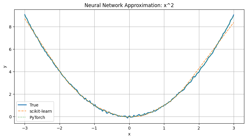

Key Takeaways

• Neural networks can learn basic mathematical functions just from data
• You don’t need to give them formulas — they learn by approximation
• This concept lays the groundwork for using neural nets in option pricing, financial modeling, and more

Up next: We’ll show how a neural net can learn to price options. Click here for that post.

A link to this notebook can be found here on GitHub