Neural Networks Part 2: Teaching a Neural Network to Price Options

In Part 1 of this series, we showed that neural networks can learn simple mathematical functions just by observing inputs and outputs — no formulas needed. But that was just warm-up.

In this post, we’ll see if a neural network can learn to price options, specifically using the Cox-Ross-Rubinstein (CRR) binomial pricing model. This takes us into quantitative finance territory — and shows how machine learning can replace traditional models.

A link to this notebook and the other notebooks can be found here on GitHub

Why This Matters

Financial models like CRR rely on mathematical assumptions about volatility, time, and risk. But they’re expensive to compute, especially at scale. What if we could train a neural net to mimic the CRR model’s outputs?

If a model can match CRR’s prices, it can serve as a fast and differentiable alternative — ideal for screeners, trading bots, and real-time tools.

The Model We’re Replacing: CRR Binomial Tree

The Cox-Ross-Rubinstein model works by simulating a tree of possible future stock prices. At each step, the stock moves up or down by a set factor. The option’s value is computed backward from expiration to the present.

It’s a powerful and interpretable model — but it’s slow if you want to compute prices for hundreds or thousands of options per second.

Inputs and Outputs

We’ll teach our neural network to predict the CRR option price based on these inputs:

Output: Option Price (as computed by the CRR model)

Step 1: Generate Synthetic Option Data

def generate_crr_dataset(n_samples=10000, option_type='call'):
    data = []
    for _ in range(n_samples):
        S = np.random.uniform(0, 150)
        K = np.random.uniform(0, 150)
        T = np.random.uniform(0.1, 2)
        r = np.random.uniform(0.0, 0.1)
        sigma = np.random.uniform(0.1, 0.5)
        N = 100  # fixed for simplicity

        price = crr_option_price(S, K, T, r, sigma, N, option_type)
        data.append([S, K, T, r, sigma, price])

    df = pd.DataFrame(data, columns=["S", "K", "T", "r", "sigma", "price"])
    return df

def generate_crr_dataset(n_samples=10000, option_type='call'):
    data = []
    for _ in range(n_samples):
        S = np.random.uniform(0, 150)
        K = np.random.uniform(0, 150)
        T = np.random.uniform(0.1, 2)
        r = np.random.uniform(0.0, 0.1)
        sigma = np.random.uniform(0.1, 0.5)
        N = 100  # fixed for simplicity

        price = crr_option_price(S, K, T, r, sigma, N, option_type)
        data.append([S, K, T, r, sigma, price])

    df = pd.DataFrame(data, columns=["S", "K", "T", "r", "sigma", "price"])
    return df

df = generate_crr_dataset(n_samples=100000, option_type='call')

X = df[["S", "K", "T", "r", "sigma"]].values
y = df["price"].values

scaler = StandardScaler()
X_scaled = scaler.fit_transform(X)

X_train, X_test, y_train, y_test = train_test_split(X_scaled, y, test_size=0.2, random_state=42)

df = generate_crr_dataset(n_samples=100000, option_type='call')

X = df[["S", "K", "T", "r", "sigma"]].values
y = df["price"].values

scaler = StandardScaler()
X_scaled = scaler.fit_transform(X)

X_train, X_test, y_train, y_test = train_test_split(X_scaled, y, test_size=0.2, random_state=42)

Step 2: Train the Neural Network

model = MLPRegressor(hidden_layer_sizes=(64, 64), activation='relu', max_iter=5000, random_state=42)
model.fit(X_train, y_train)

y_pred = model.predict(X_test)
mse = mean_squared_error(y_test, y_pred)
print(f"Test MSE: {mse:.4f}")

model = MLPRegressor(hidden_layer_sizes=(64, 64), activation='relu', max_iter=5000, random_state=42)
model.fit(X_train, y_train)

y_pred = model.predict(X_test)
mse = mean_squared_error(y_test, y_pred)
print(f"Test MSE: {mse:.4f}")

Step 3: Evaluate the Results

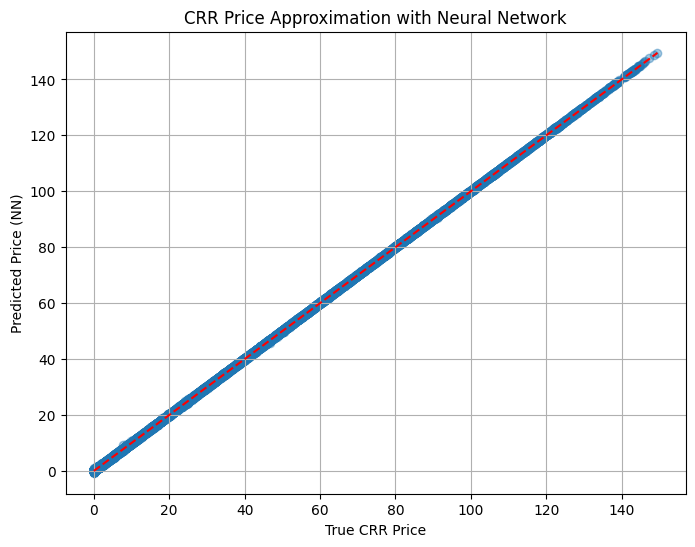
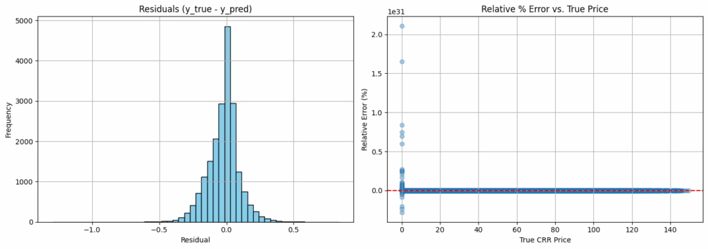
📊 RMSE: 0.1180
📊 MAE: 0.0837
📊 Average % Error: 0.85%

Yes — that’s a model that can mimic CRR pricing with sub-$0.10 average error across thousands of option scenarios.

Step 4: Save for Reuse

# Save the model and scaler
import joblib

# Save trained model
joblib.dump(model, "nn_crr_model.pkl")

# Save the scaler (used to transform inputs)
joblib.dump(scaler, "nn_crr_scaler.pkl")

print("✅ Model and scaler saved to disk.")

# Save the model and scaler
import joblib

# Save trained model
joblib.dump(model, "nn_crr_model.pkl")

# Save the scaler (used to transform inputs)
joblib.dump(scaler, "nn_crr_scaler.pkl")

print("✅ Model and scaler saved to disk.")

You’ll use these in the next step when analyzing real options.

Key Takeaways

• CRR is a reliable pricing model — but computationally expensive
• Neural networks can replicate CRR results with excellent accuracy
• Once trained, the NN is much faster than computing the binomial tree repeatedly

In the next post, we’ll use this trained model to scan real option chains (like PLTR) and find mispriced vertical spreads.

A link to this notebook can be found here on GitHub